Multi-armed bandit - optimistic initial values

May 28, 2017 · 3 min read

This post is part of my struggle with the book "Reinforcement Learning: An Introduction" by Richard S. Sutton and Andrew G. Barto. Other posts systematizing my knowledge and presenting the code I wrote can be found under the tag Sutton & Barto and in the repository dloranc/reinforcement-learning-an-introduction.

All the methods I have described so far depend on initial estimates of the value of $Q_1(a)$ . This is especially visible when we calculate MAB with $\epsilon = 0$ , i.e. without exploration, still selecting the best possible action (arm). In statistics, we call such methods biased. The bias disappears for methods with $\alpha$ of $\frac{1}{n}$ when each action is selected at least once. For constant $\alpha$ , the bias does not disappear, it only decreases with time (subsequent iterations of the algorithm).

To get rid of the bias, we can use something like optimistic initial values. In the code of the examples I have written so far, the true values of each action came from the normal distribution (mean 0, variance 1) and were set in the constructor:

self.true_reward = [np.random.randn() for _ in range(self.arms)]

By the way, I would like to remind you that getting the value for a given action looks like this:

def get_reward(self, action):
    return self.true_reward[action] + np.random.randn()

That's it for the reminder.

We can encourage the algorithm to explore at the beginning of its operation by setting very optimistic initial values. I chose the number 5 and it looks like this:

self.action_count = np.ones(self.arms)

self.rewards = np.ones(self.arms) * 5

And that's it, no more modifications to the code are needed. What happens when we run the script with such self.rewards values? Let's see this with an example with epsilon equal to zero:

self.rewards:
[ 5.  5.  5.  5.  5.  5.  5.  5.  5.  5.]

reward: 1.87411213524
[ 3.43705607  5.          5.          5.          5.          5.          5.
  1.          5.          5.        ]
reward: 0.504446069392
[ 3.43705607  2.75222303  5.          5.          5.          5.          5.
  1.          5.          5.        ]
reward: 0.374953664141
[ 3.43705607  2.75222303  2.68747683  5.          5.          5.          5.
  1.          5.          5.        ]
reward: -3.66371477543
[ 3.43705607  2.75222303  2.68747683  0.66814261  5.          5.          5.
  1.          5.          5.        ]
reward: -1.59327852639
[ 3.43705607  2.75222303  2.68747683  0.66814261  1.70336074  5.          5.
  1.          5.          5.        ]
reward: -2.41539982786
[ 3.43705607  2.75222303  2.68747683  0.66814261  1.70336074  1.29230009
  1.          5.          5.          5.        ]
reward: -0.641184621377
[ 3.43705607  2.75222303  2.68747683  0.66814261  1.70336074  1.29230009
  2.17940769  5.          5.          5.        ]
reward: -1.53850026836
[ 3.43705607  2.75222303  2.68747683  0.66814261  1.70336074  1.29230009
  2.17940769  1.73074987  5.          5.        ]

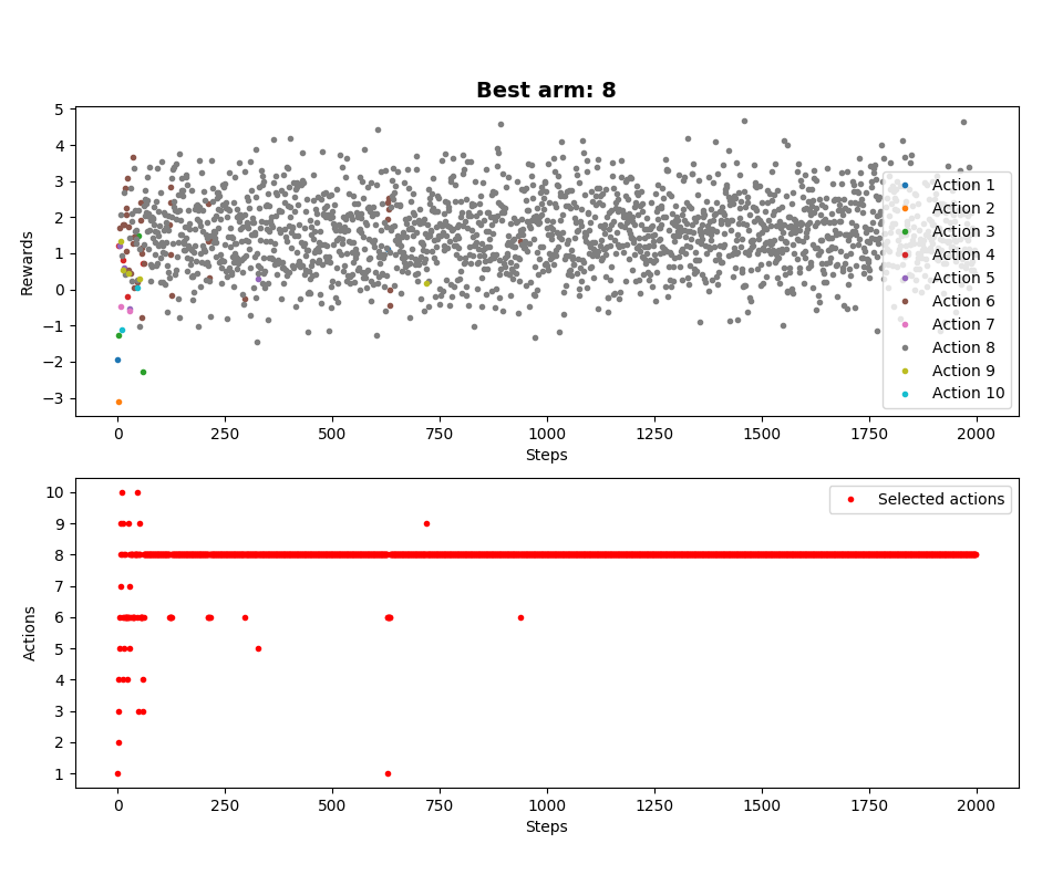
The rewards received are less than five and averaged, so even for an epsilon of zero, exploration occurs and the algorithm tries each action in turn. Let's see it graphically (epsilon equal to zero):

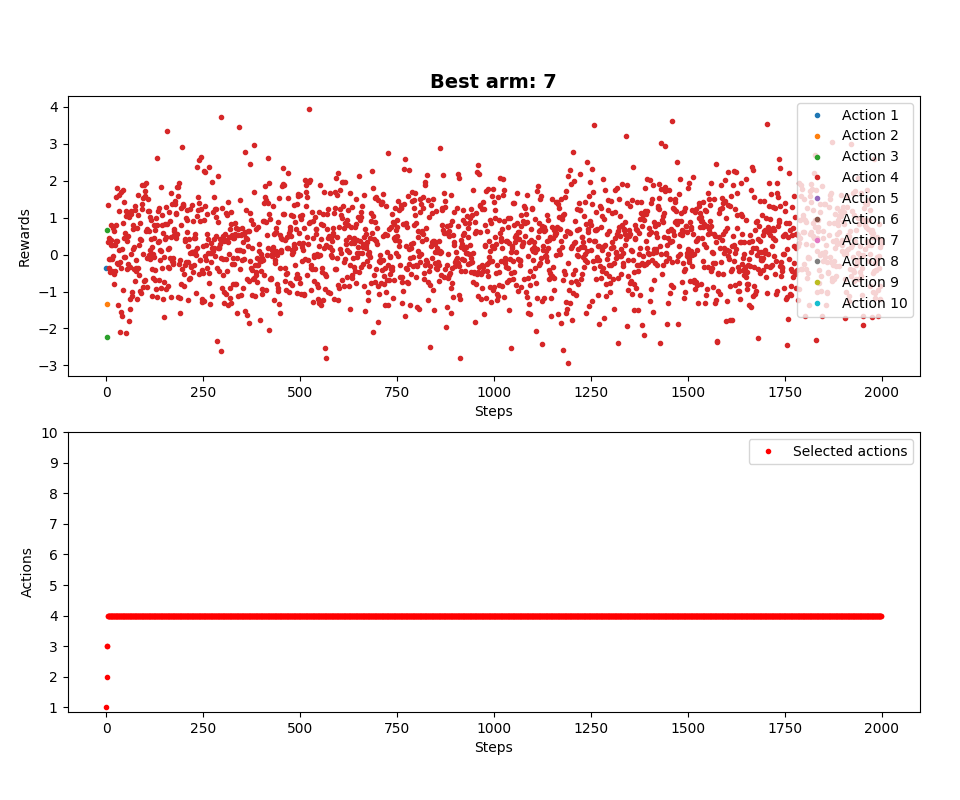
optimistic initial values, epsilon = 0

For comparison, without our optimization (epsilon is also zero):

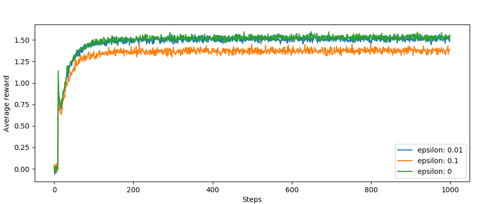
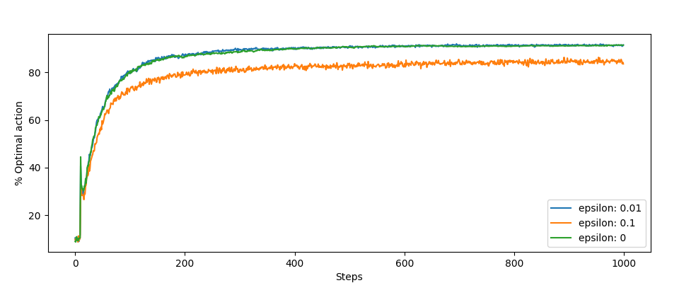
bez optimistic initial values, epsilon = 0

The other charts, those jumps at the beginning are interesting. This is the result of our optimization:

średnie nagrody optymalne akcje

Summary

As you can see, this is a simple but quite effective way to encourage MAB with e-greedy strategy, even as it selects the best actions every time. However, this method only works at the beginning of the algorithm, during the first dozen or so iterations. In the next post I will deal with a way to improve exploration, the so-called Upper-Confidence-Bound method.

Summary​

Summary